1.3: The need for detailed and complex simulations
Here we're going to try to look at climate effects under different feedback assumptions.
Let’s quickly set the scene in terms of where we are emission wise and what this means. In pre-industrial times CO₂ concentration was around 278 parts per million (ppm) today we are around 408ppm. This increase is what’s causing all of our problems. For context 1ppm is roughly equivalent to 2.13Gt of Carbon or 7.8Gt of CO₂. Because of absorption dynamics it’s not actually enough to remove this amount of CO₂ to drop down a ppm, we would probably have to remove around twice as much, so if we want to drop 1ppm we would have to remove around 15Gt of CO₂.
One approach for ball-parking the feedback effects, outside of complex, many-parameter, simulations, is to look at the past.
I'm going to put below the equation we're working towards, don't worry if it looks like a lot we're going to go through the derivations in more detail below:
Interestingly, the logarithmic dependence of ΔF on CO₂ concentration is predicted from complex global simulations, but the basic physical reasons do not seem to be completely trivial:
Ignoring feedback
This section was inspired by this site.Let’s start by just considering the direct adsorption of the outgoing infrared by CO2 itself. From a simple calculation using the radiation balance physics we’ve discussed already the change in temperature for a given amount of radiative forcing is:
ΔF is the radiative forcing from additional greenhouse gasses relative to those in pre-industrial times
Tp is the planetary surface temperature prior to additional greenhouse gasses being added ~ 288 Kelvin
A ~ 0.3 is the albedo
S is the average solar flux incoming, namely 1/4 of our 1376W/m^2 from above.
If we plug this in we get the 0.3 Kelvin/Watt/Meter² term from the above formula.
Second, we have to get the radiative forcing ΔF from the CO2 concentration. The 5.35 Watt per meter squared and the logarithmic dependence comes from the IPCC form used here.
If we plug this equation into an online plotter, this gives the following curve:

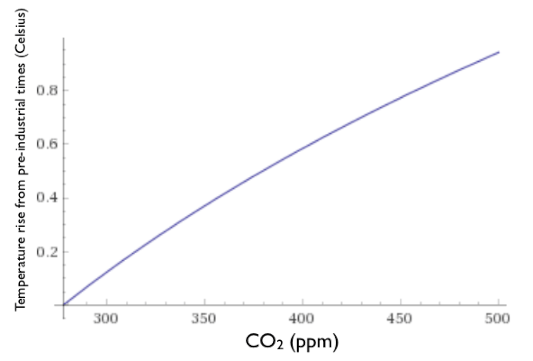
Plugging in our current 408 ppm to the above logarithmic formula, we get 0.6K of warming from pre-industrial times, versus around 1K observed in actual reality. This gives us something to compare against but is not the right curve for this relationship in reality. In addition to not including any feedback our model is also neglecting other greenhouse gasses.
One issue is that the absorption of infrared radiation by CO2 is associated with broad spectral bands and sidebands, and at the peaks of those absorption bands, absorption is saturated from the beginning — i.e., essentially every outgoing infrared photon from the surface with a wavelength right in the center one of these peaks will definitely be absorbed by CO2 long before it exits the atmosphere, even at pre-industrial CO2 concentrations — while regions near but not quite at the peaks may become saturated with increasing CO2 concentration.
Another key issue has to do with the height in the atmosphere from which successful radiation out to space occurs, and hence with the temperature at which it occurs — given the Stefan-Boltzmann T^4 dependence of the emitted radiation, and the fact that temperature drops off sharply with height into the atmosphere, the rate of radiation will depend strongly on the height of the source in the atmosphere.
If newly added CO2 effectively absorbs and emits IR radiation from higher in the atmosphere, its contribution to the outflux term of the radiative balance will be smaller, warming the planet, but this dependence needn’t be linear on the CO2 concentration and in fact can be logarithmic. A bit more precisely, adding more CO2 to the atmosphere causes the height at which successful emission into space occurs to move higher, and hence colder, and hence *less*. It intuitively does, which this wonderful paper explains from the perspective of convection in the atmosphere: “the planetary energy balance is not purely radiative but is mediated by convection, with water vapor as the key middleman”.
With a historical estimate of feedback
However, importantly, the formula we just used, which doesn’t take into account any kind of water vapor or biological feedbacks, not to mention many others, underestimates certain longer-timescale historical data, taken from a record that spans over tens of thousands of years, by about a factor of about 4.
As the ACS website puts it:
The sensitivity factor this talks about is the term out front of the logarithmic expression for temperature change versus CO2 concentration
our calculated temperature change, that includes only the radiative forcing from increases in greenhouse gas concentrations, accounts for 20-25% of this observed temperature increase. This result implies a climate sensitivity factor perhaps four to five times greater, ∼1.3 K·(W·m–2)–1, than obtained by simply balancing the radiative forcing of the greenhouse gasses. The analysis based only on greenhouse gas forcing has not accounted for feedbacks in the planetary system triggered by increasing temperature, including changes in the structure of the atmosphere.
So what happens if we put in the missing factor of 4? Then the formula will be:
This looks like:
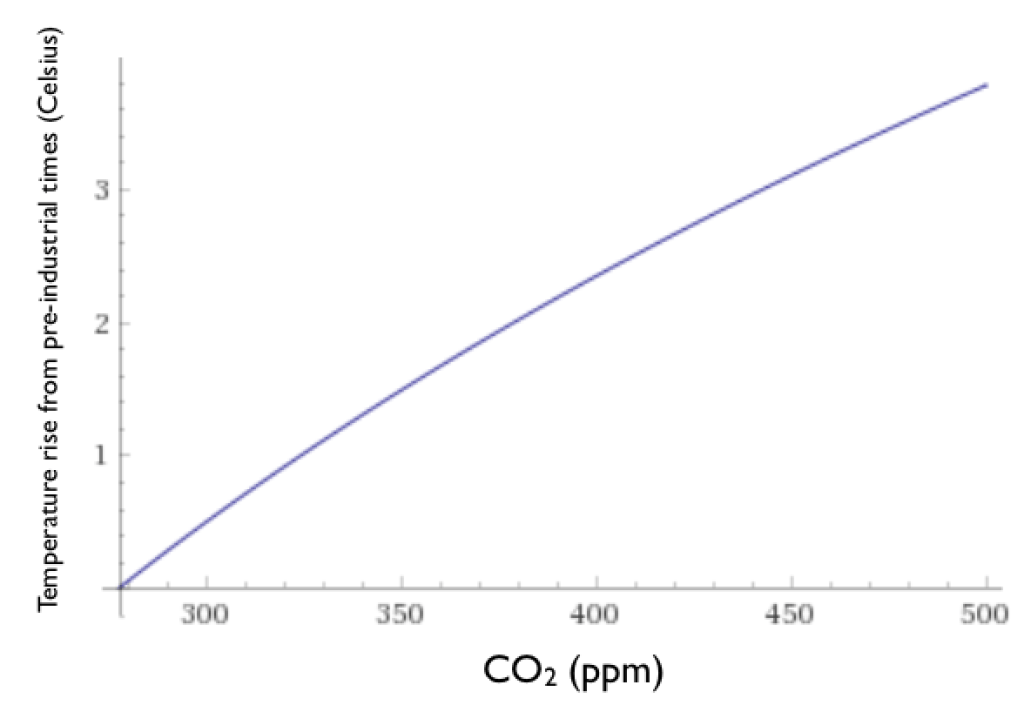
Then, even at our current ~408 ppm CO2 concentration, we would expect 2.4℃ of warming to ultimately (once the slow feedbacks catch up) occur, relative to pre-industrial times
Now, this is much more warming than has occurred so far. What to make of that? Well, as mentioned above, the water-based feedback phenomena can take decades to manifestgiven for instance the large heat capacity of the oceans, so perhaps we should not be surprised that the temperature of the Earth has not yet caught up with where it is going to be heading over the coming decades, even for a hypothetical fixed amount of CO2 from now on, according to this formula.
A recent paper tried to pin down the magnitude of the water feedback based on more recent, rather than long-term historical, observations, including measurements of the water vapor concentration itself. They concluded that the missing feedback factor might be closer to 2, rather than the 4 above.They do add the caveat that they because of the shortness of their observations, 7 years, there is some inevitable confidence intervals around this value. Either of these values still means though that unless the ppm of CO₂ in the atmosphere falls quickly things are not looking good
Potential tipping points
Some have argued that a nominal 2C target, given comparatively fast feedbacks like water vapor, actually corresponds to a nearly inexorable push to 3C or higher long-term when slower feedbacks are taken into account.Alas, fitting historical or even quite recent data for the “missing feedback factor” isn’t really fully predictive either, even if we had enough of that data, due to abrupt phase transitions or tipping points which can occur at different temperatures. For example, rapid one-time arctic methane release from the permafrost, or ocean albedo decrease brought on by sea ice melting.
To be sure, many seem to disagree that the relevant tipping points are likely to be around 2C, as opposed to higher.As explained here Here is a nice thread about the significance or lack thereof of current targets like 2℃ or 1.5℃ from a tipping point perspective. Also, many tipping points would take decades or centuries to manifest their effects, giving time for response, and in some cases in principle for reversal by bringing temperature back down through negative emissions.
We should probably also worry about nonlinear effects that would depend on the rate of change or the variance of of climate variables. For instance if ecologies can adapt to a given change over long timescales but struggle to do so over short timescalesBut on the more worrisome side, I have seen plenty of papers and analyses that do point to the potential for major tipping points / bi-stabilities around 2℃, or sometimes even less. For example, this paper uses 2℃ as a rough estimate of the temperature that you don’t want to exceed for risk of hitting a potential cascade of major tipping points. Likewise this analysis points to potential tipping points in arctic permafrost methane release at even lower temperatures.
A middle of the road climate sensitivity
For comparison, using sophisticated climate models, plus models of the human activity, IPCC projects 2-4℃K of warming by 2100Our climate curves give this equivalence when the feedback factor is around 2.5 (rather than the 4 we initially used).
There is no reason that the curve with feedback has to be a simple multiple of the curve without feedback, i.e., that there is any simple “missing factor” at all, as opposed to a totally different shape of the dependency. Indeed, in scenarios with large abrupt tipping points this would certainly not be the case. You do, however, get something similar to this description when you linearize simple ordinary differential equation models for the planetary energy balance, by assuming a small perturbation around a given temperature — this is treated here. The site just linked arrives at a temperature perturbation deltaT ~ -R/lambda, where R is the radiative forcing and lambda is a feedback factor that arises from the linearization. In their analysis, they get lambda = −3.3 W m^-2 K^-1 due to just the direct effects of the CO2 forcing and blackbody radiation (called Planck forcing) and lambda = -1.3 W m^-2 K^-1 in a middle of the road IPCC climate sensitivity estimate: I think it is not coincidental here that -3.3/-1.3 ~ 2.5, which is the same as our “missing feedback factor” for the IPCC climate sensitivity estimate just above. In any case, the analysis here gives a more rigorous definition of feedback factors in linearized models and how to break them down into components due to different causes.)
TRCE stands for the transient climate response to cumulative carbon emissions, which is the ratio of global average surface temperature change per unit of CO₂ emittedWe can also try to crudely translate this into the TCRE measure used in the IPCC reports
A classic meme is that 450 ppm ~ 2℃. This would translate into a TCRE of 2.7C/1000PgC. The IPCC states, based on statistically aggregating results of complex simulations and so forth, a likely range for the TCRE of 0.8 to 2.5C/1000PgC with a best observational estimate of 1.35C/1000PgC, suggesting that our feedback factor of 2.5 may be a bit high and a feedback factor of 2 may be more appropriate as a middle of the range estimate.
Implications for carbon budgets
Potential tipping points
What would this particular curve, with the “feedback factor” of 2.5, imply for the hypothetical scenario where we abruptly ceased emissions quite soon?
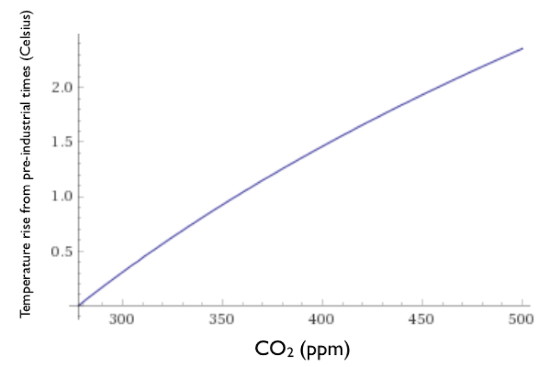
Per the curve, we’d still potentially be looking at around 1.5C of ultimate warming (due to feedbacks), with roughly our current atmospheric CO2 levels kept constant.
With the feedback factor of 2 instead of 2.5, we’d cross 1.5C at around 440 ppm, and our remaining carbon budget for 1.5C at the time of writing would therefore be around 2*(440-405 ppm)*7.81=547Gt CO₂ emitted.
See slide 15 there
For more good discussion here and hereFor comparison, one figure I’ve seen gives around 0.1C per decade of additional warming even under year 2000 atmospheric CO2 levels kept constant, although another analysis suggests roughly constant temperature (little further warming) if carbon emissions were to completely and abruptly cease — these are not inconsistent, since if emissions somehow completely ceased, natural carbon sinks could start to kick in to slowly decrease atmospheric CO2, which is not the same as holding CO2 concentrations constant.
It is not obvious to me a priori that some fixed amount of CO2 added to the atmosphere would be naturally removed, on net, at all, even on long timescales… a carbon cycle could in principle keep atmospheric CO2 at a stable level that simply happens to be higher than the pre-industrial concentration. But according to a nice discussion in the introduction to the NAS report on negative emissions, the sinks are real and active, and indeed once human emissions fall low enough, not even necessarily to zero, the sinks can bring the rate of change of atmospheric CO2 concentration to net negative:
To reduce atmospheric CO2 from 450 to 400 ppm, it would not be necessary to create net negative anthropogenic emissions equal to the net positive historical emissions that caused the concentration to increase from 400 to 450 ppm. The persistent disequilibrium uptake by the land and ocean carbon sinks would allow for achievement of this reduction even with net positive anthropogenic emissions during the 50 ppm decline.
See here for a much better analysis
Even some of the scenarios that target 1.5C set that as an ultimate target for the end of the century, and actually slightly exceed that target between now and then, relying on negative emissions to bring it down afterwards. This recen t Nature paper though explains the dangers of thinking this wayAnyway, loosely speaking,from what I’ve understood, in the absence of large-scale deployment of negative emissions technology, it seems unlikely that we have more than 10 years of emissions at current levels while still having a high likelihood of not exceeding a 1.5C peak warming, given what we know now. That’s ~400 GigaTonnes CO2 for the 10 years, versus a budget of roughly zero for a feedback factor of 2.5 and roughly 550Gt CO₂ for a feedback factor of 2 as estimated above. There is a chance we’ve already committed to 1.5C peak warming, in the absence of large-scale negative emissions, regardless of what else we do.
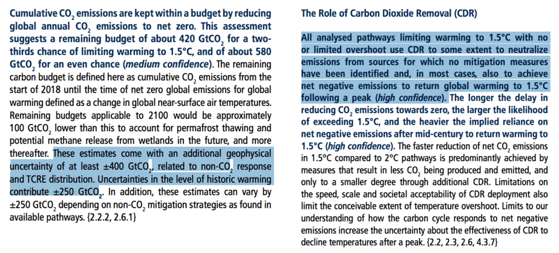
With all that in mind, here are two snippets from the IPCC report on 1.5C (written over a year ago so the carbon budget is roughly 40-80 Gt CO₂ less now). The left hand snippet expresses the level of uncertainty in the remaining carbon budget for 1.5C, and the right snippet mentions the need for negative emissions in real-world scenarios where we stabilize to 1.5C. Their 420-580 Gt CO₂ budget from a year or so ago accords decently well with what we got (zero to 550 Gt CO₂) from the feedback factor of 2-2.5 case above.

Again, subject to all the caveats about the notion of carbon budgets here, not to mention our crappiest of models.
At the time of writing, meanwhile, this calculator from the Guardian, gives 687 GigaTonnes, or 17 years at our current emissions rateWe can also ballpark a remaining carbon budget for 2℃ warming using the 450 ppm ~ 2℃ idea.
450 ppm ~ 3514 Gt of CO2 in the atmosphere, versus ~3163 Gt (405 ppm) up there now, so we would be allowed to add around 300 or 350 more. So if the oceans and land plants absorb 1/2 of what we emit (bad for ocean acidification), the maximum carbon budget for 2℃ in this very particular scenario is around 2*(3514-3163) GigaTonnes CO2 = 702 GigaTonnes of emitted CO2 if there are no negative emissions.
2*(480-405 ppm)*7.81 Gt CO₂/ppm = 1171 Gt CO₂,
Or if we use 530 ppm as our 2℃ target we get 2*(530-405)*7.81=1953 Gt CO₂Now, the carbon budgets I’m seeing in the IPCC reports for 2℃ seem a bit higher, in the range of 1200-2000 GigaTonnes, which we can get if we use 480 ppm as our target for 2℃ instead of 450 ppm.