1.2: Climate sensitivity
¹ effective ε and A (and f) in the above formulaA key further problem for us as back-of-the-envelope-ers, though, is to know what a given amount of CO2 in the atmosphere translates to in terms of the amount of warming¹. This is where things get trickier. Before trying to pin down a number for this “climate sensitivity”, let’s first review why doing so is a very complex and multi-factorial problem.
Water vapor
² i.e more absorbed outgoing radiation
If you just consider clouds per se, it looks like they on average cool the Earth, from an experiment described in lecture 10a of the Caltech intro course, but this depends heavily on their geographic distribution and properties., The PICC reports state directly that this area is of limited scientific understanding
Some further links:
Earth’s outgoing longwave radiation linear due to H2O greenhouse effect
How Earth sheds heat into space
Even weirder,
Global warming increased solar radiation
Shortwave and longwave radiative contributions to global warming under increasing CO2Naively, if we think of the only effect of CO2 as being the absorption of some of the outgoing infrared thermal radiation from the planet surface, then more CO2 means higher ε ², with no change in albedo A. However, in reality, more warming also leads to more water vapor in the atmosphere, which — since water vapor is itself a greenhouse gas — can lead to more greenhouse effect and hence more warming, causing a positive feedback. On the other hand, if the extra water vapor forms clouds, that can increase the albedo, decreasing warming by blocking some of the incoming solar radiation from hitting the surface, and leading to a negative feedback. So it doesn’t seem obvious even what functional form the impact of CO2 concentration on ε and A should take, particularly since water vapor can play multiple roles in the translation process.
The roles of carbon dioxide and water may be such that the largest warming mechanism is increased penetrance of solar radiation rather than decreased escape of infrared per se. As the article explains:
While one would expect the longwave radiation that escapes into space to decline with increasing CO2, the amount actually begins to rise. At the same time, the atmosphere absorbs more and more incoming solar radiation; it’s this enhanced shortwave absorption that ultimately sustains global warming.”
Moreover, the feedback effects due to changes associated with water take a long time to manifest, due in part to the large specific heat of water and the large overall heat capacity of the enormous, deep oceans, and in part due to the long residence time of CO2 in the atmosphere. Thus, simply fitting curves for observed temperature versus CO2 concentration on a short timescale around the present time may fail to reflect long-timescale processes that will be kicking in over the coming decades, such as feedbacks.
All this is to say that the feedback mechanisms between CO₂ and water vapor are very tricky to model.
Ocean biology effects
It isn’t quite as clear cut as this though as the magnitude of this effect is hard to pin down, even whether it always leads to less CO₂ drawdown is an open question.There are also large ocean biology and chemistry effects. Just to list a few, dissolved carbon impacts the acidity of the ocean, which in turn impacts its ability to uptake more carbon from the atmosphere. There are also major ocean biological effects from photosynthesis and the drivers of it. Roughly, as this Caltech course explains when water from the deep ocean mixes with surface water it can stimulate organic growth drawing down carbon. Global warming however can have the effect of reducing this mixing, reducing ocean CO₂ uptake.
The oceans sequester around 100Gt a year (very similar to land) with a significant part of the long-term sequestration of carbon going to the deep ocean due to settling of biological material under gravity and other mechanisms.
Land biology effects
There are also terrestrial biological effects.
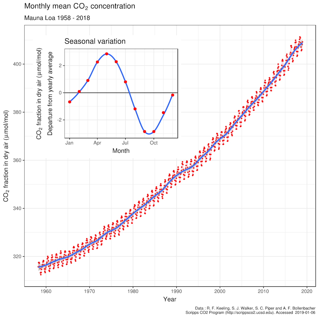
Dyson is known as a bit of a “heretic” on climate and many other topicsIn 1977, in a paper that will come up again for us in the context of carbon sequestration technologies, Dyson pointed out that the yearly photosynthetic turnover of CO2, with carbon going into the bodies of plants and then being released back into the atmosphere through respiration and decay, is >10x yearly industrial emissions. The biological turnover is almost exactly in balance over a year, but not perfectly so at any location and instant of time. The slight imbalances over time give the yearly oscillation in the Keeling curve:
Recently, this paper measured the specifics on land, concluding “150–175 petagrams of carbon per year” of photosynthesis, whereas global emissions are roughly ~10 petagrams (gigatonnes) of carbon each year (~40 of CO2).

Dyson goes on to discuss potential ways to tip the balance of this large swing towards net fixation, rather than full turnover, which he suggests to do via a plant growing program — we’ll discuss this in relation to biology-based carbon sequestration concepts later on.Dyson stressed that any net imbalances that arise in this process, e.g., due to “CO2 fertilization” effects — which cause increased growth rate or mass of plant matter with higher available atmospheric CO2 concentration — could exert large effects.
Measurements of CO2 fertilization of land plants have improved since Dyson was writing, e.g., this paper, which gives a value: “…0.64 ± 0.28 PgC yr−1 per hundred ppm of eCO2. Extrapolating worldwide, this… projects the global terrestrial carbon sink to increase by 3.5 ± 1.9 PgC yr−1 for an increase in CO2 of 100 ppm“. That is pretty small compared to emissions.
This diagram (a bit out of date on the exact numbers) summarizes the overall pattern of ongoing fluxes in the carbon cycle
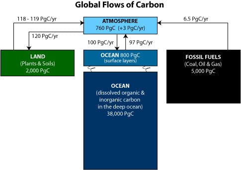
And here is a nice animation of this over time as emissions due to human activity have rapidly increased.
Permafrost
Eli Dourado covers the fascinating Pleistocene Park project which aims to influence this. There are also surprisingly wildfire risks to these areas.There are other large potential feedback effects, beyond those due to water vapor or plant life, e.g., over 1000 gigatonnes of carbon trapped in the arctic tundra, particularly in the form of the greenhouse gas methane which exerts much stronger short term effects than carbon, and which could be released due to thawing of the permafrost.
Local warming
While we often hear about global temperature rises this somewhat obscures the fact that global warming effects different geographies and climates to vastly different degrees. As Dyson emphasizes:
The effect of carbon dioxide is important where the air is dry, and air is usually dry only where it is cold. Hot desert air may feel dry but often contains a lot of water vapor. The warming effect of carbon dioxide is strongest where air is cold and dry, mainly in the arctic rather than in the tropics, mainly in mountainous regions rather than in lowlands, mainly in winter rather than in summer, and mainly at night rather than in daytime. The warming is real, but it is mostly making cold places warmer rather than making hot places hotter.
If you want to see which places this effect leads to being hit the worst this map shows it off well.

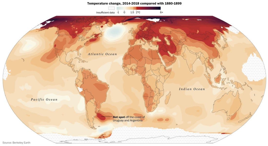
Michael Mann’s online course has a nice lecture on a simple model of the climate system that includes a latitude axis.Note the darker red up by the Arctic. Note also that spatial non-uniformities in temperature, between locations on the globe, as well as the temperature changes between the surface and the atmosphere, are a major driver of weather phenomena.
Heat stress
One worry that is a bit less about the climate and a bit more about the climate’s effects on us is heat stress. A recent paper takes a look at what climate scenarios might put a vast number of humans at risk. The key metric here is to look at wet bulb temperatures, this basically describes the minimum temperature a human body can get to under ambient conditions. Or put another way if you are just standing around and sweating what is the lowest your body temperature will get to.
Any wet bulb temperature above 31℃ poses extreme risks to human welfare and conditions over 35℃ leads to significant risk of hyperthermia. The paper goes on to say that while these conditions do not exist in an extended way anywhere today they “would begin to occur with global-mean warming of about 7 °C, calling the habitability of some regions into question. With 11–12 °C warming, such regions would spread to encompass the majority of the human population as currently distributed”.
These might seem like very high levels of warming but they correspond to bad case scenarios in the IPCC report models and so are noth thought to be totally out of consideration. The paper mainly acts as a warning that the effects of the higher temperature futures might be significantly worse than people typically think.
____________________________________________